
Problem:
The objective is to determine if the EMS calls and false alarms for Fort Worth Fire Department Battalion 2 exhibit clustering, and to assess the level of clustering so that education programs can be used in areas with high false responses, and EMS response station can be placed into areas with lots of calls.
Analysis Procedures:
average nearest neighbor tool : This calculates an index based on how close features are located and compares that distance to an index for randomly distributed features. This assesses clustering by location only. The tool is used by inputting the feature class of interest (False incident types 700-745) and setting the area to a size similar to the dataset (area of battalion 2). This analysis used the definition query to highlight only incident types between which were false alarms.
High/Low Clustering: The Getis-Ord General G tool examines clustering by value. The tool determines whether areas of similar values are more clustered than would be expected in a random distribution. To use this tool, the dataset must first be examined for the approximate number of neighbors and the distance band. Initial distance band was set using the average distance between points (around 1000), and distance bands increases from 200 feet to 1200 feet in 200 foot intervals. This helps determine the distance range to use (the one with the highest z value) for the January 2007 EMS calls.
multi-distance clustering tool: Ripley’s K function is similar to the nearest neighbor calculation, but can also examine multiple distances and factors other than the next nearest feature. This tool requires the layer of interest (January EMS 2007 Calls), number of distance bands (200 ft at 100 foot intervals), and also the number of confidence envelopes that should be used (99 permutations). The confidence envelope is a permutation of the random distribution used for comparison. The results are displayed graphically as a comparison between observed and expected results. An area used is the minimum enclosing rectangle.
Spatial Autocorrelation Tool : The global Moran’s I combines evaluation of clustering by location and value. This tool requires a layer and field of interest (February 2007 EMS Calls), but also requires that a grid cell size be chosen (spatial join of the map area of interest to 200 square foot cells). Remove grid values with 0 values using a definition query. Run the spatial autocorrelation between 250-600 feet in 50 foot increments to find the maximum z score.
An example flow diagram is represented in Figure 1.
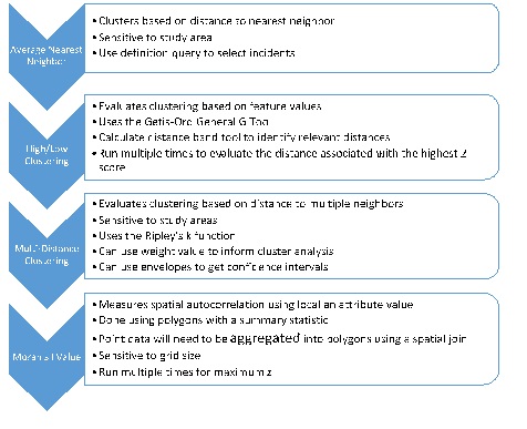
Figure 1: Flow diagram of the spatial pattern analysis.
Results:
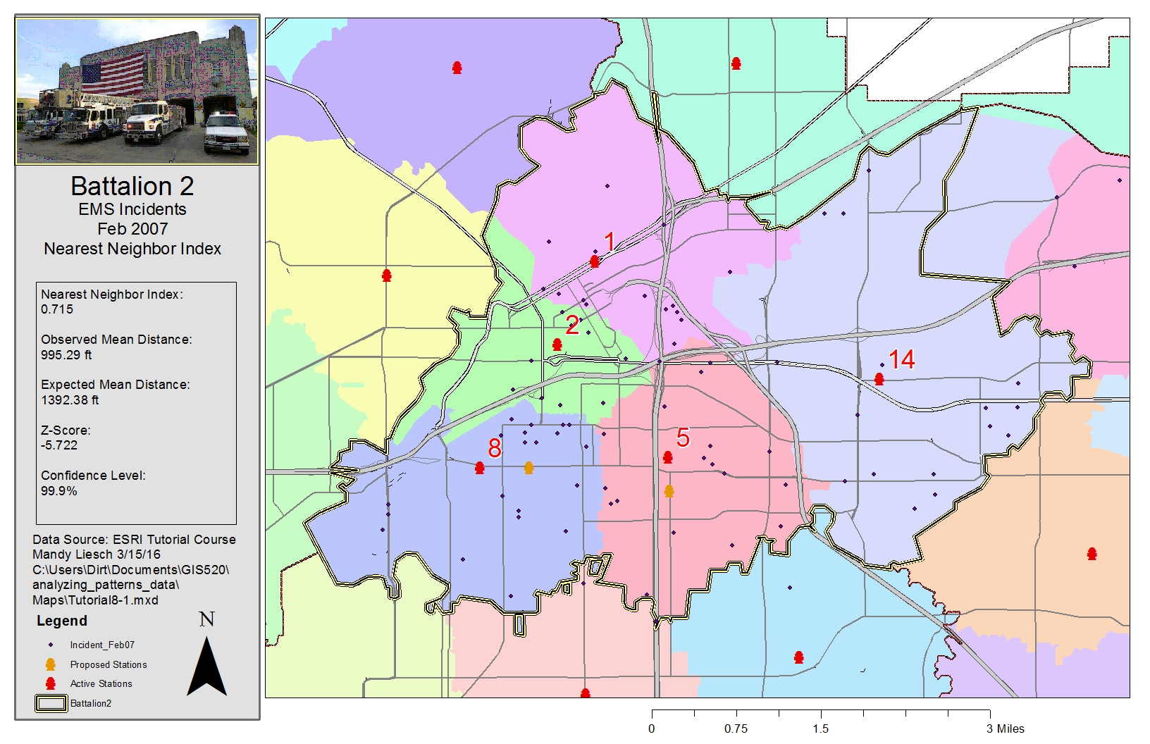
Figure 2: Figure 2. Results of using the nearest neighbor methods to calculate an index and z-score to determine clustering. Click on map for enlarged image.
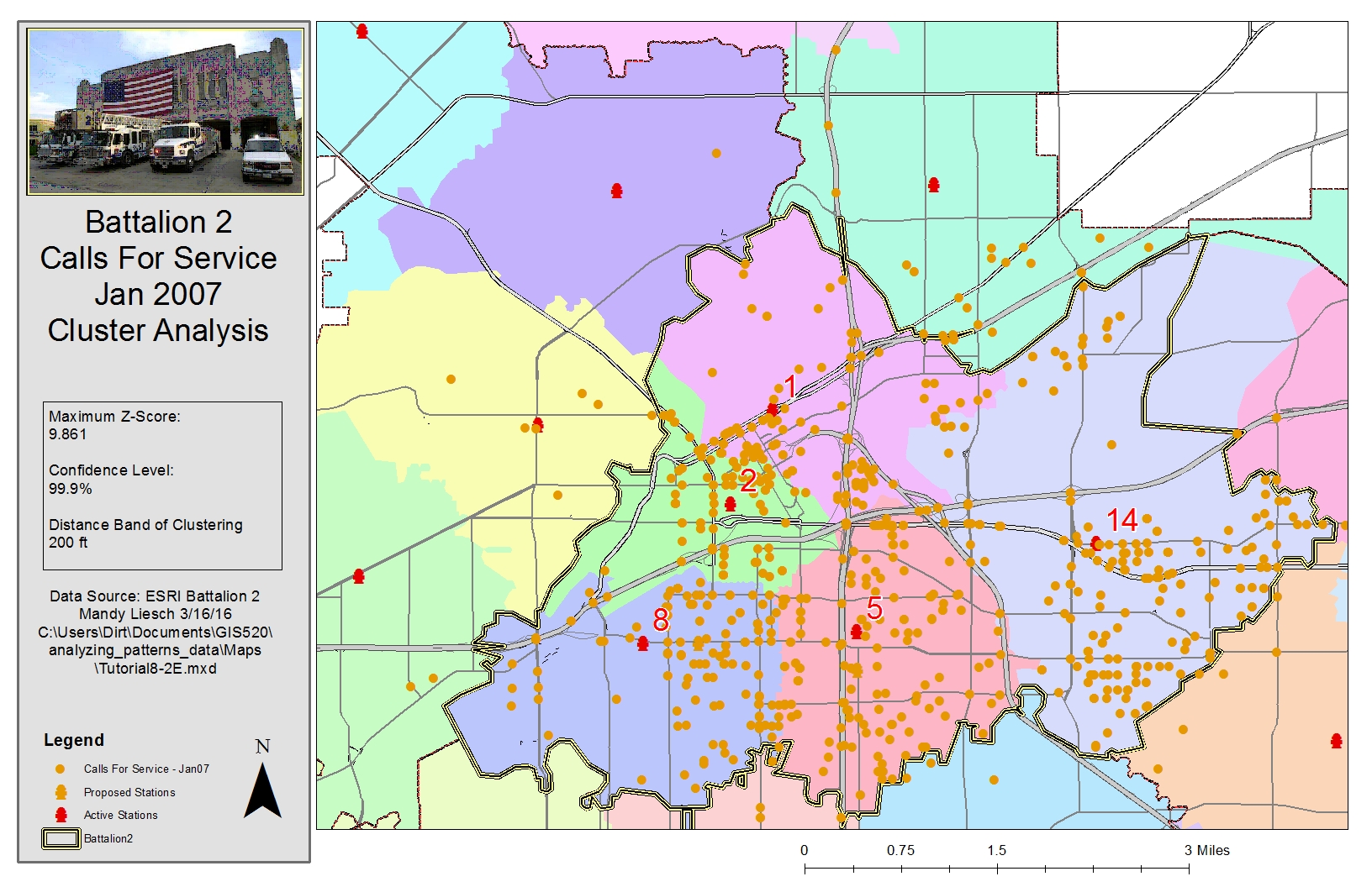
Figure 3. Results of using the Getis-Ord General G tool to calculate a z-score to assess whether the features were clustered. Click on map for enlarged image

Figure 4. Results of using the multi-distance spatial cluster analysis tool (Ripley’s K Function) to assess the significance of clustering. Click on the map for an enlarged image.

Figure 5. Results of using the spatial autocorrelation tool (Global Moran’s I) to determine z-scores and confidence levels assessing the level of clustering at varying distances (based on an initial 200-foot grid). Click on the map for an enlarged image.
Application & Reflection:
Spatial autocorrelation is critically important in a lot of different aspects of farm marketing and optimizing farm production. We can use our customer purchasing demographics to determine if our customers are located in a cluster. We can then target our marketing campaign to these areas. We can also look at regional purchasing patterns of us, and the purchase patterns of our competitors. This gives us data we can use to target grocery stores and restaurants in these areas with a loyal customer base.
Problem description: Our dairy goat operation relies on using several different pastures. We can study the overall biomass yield, and use these clusters to try and find which environmental factors contribute to the higher overall pasture production.
Data needed: We need pasture biomass yield (measured by us), soil tests, soil moisture, rainfall, etc.
Analysis procedures: We can also use the Ripley’s K function to identify the clustering of plant species across all of the pastures, targeting spread of weeds, or beneficial plants. We can also examine milk yield for dairy goats on different pastures. This way, we can use spatial autocorrelation to find clusters of high producing does, and study vegetation and water type in the area.
